
Convolutional neural network retrieval#
Convolutional neural networks (CNNs) make it easy to leverage the additional structural information in the spatial retrieval input data for retrieving precipitation. This model demonstrates this using a basic UNet model.
NOTE: This notebook can be run on Google Colab. To install the necessary dependencies uncomment the following cell and execute it.
#!pip install satrain[complete]
The training data#
The satrain package provides two PyTorch dataset to access the SatRain data: One for tabular and one for spatial. The term spatial is used here to denote input data in 2D or image structure.
The satrain.pytorch.dataset.SatRainSpatial implements the PyTorch dataset interface for loading SatRain data in spatial format.
For the CNN-based retrieval we use the gridded geometry. Apart from that we choose retrieval input and target configuration similar to those in the fully-connected NN example.
%load_ext autoreload
%autoreload 2
from satrain.input import GMI, Ancillary, Geo, GeoIR
from satrain.target import TargetConfig

target_config = TargetConfig(min_rqi=0.5)
inputs = [GMI(normalize="minmax", nan=-1.5, include_angles=False)]
geometry = "gridded"
With these settings, we can instantiate the training data dataset. By setting stack=True we also tell the retrieval to stack all input tensors instead of loading the input data as a dictionary.
from torch.utils.data import DataLoader
from satrain.pytorch.datasets import SatRainSpatial

batch_size = 32
training_data = SatRainSpatial(
    base_sensor="gmi",
    geometry=geometry,
    split="training",
    subset="xs",
    retrieval_input=inputs,
    target_config=target_config,
    stack=True,
    download=True,
)
training_loader = DataLoader(
    training_data,
    shuffle=True,
    batch_size=batch_size,
    num_workers=8,
    worker_init_fn=training_data.worker_init_fn,
    pin_memory=True
)
With the above configuration, the training data loaded by the training_loader has the following dimensions.
inpt, target = next(iter(training_loader))
print("Input tensor shape: ", inpt.shape)
print("Target tensor shape: ", target["surface_precip"].shape)
Input tensor shape:  torch.Size([32, 13, 256, 256])
Target tensor shape:  torch.Size([32, 256, 256])
For the validation, we instantiate dataset and dataloader with the same settings but choose the validation split instead of the training split.
validation_data = SatRainSpatial(
    base_sensor="gmi",
    geometry=geometry,
    split="validation",
    subset="xs",
    retrieval_input=inputs,
    target_config=target_config,
    augment=False,
    stack=True,
    download=True,
)
validation_loader = DataLoader(
    validation_data,
    shuffle=False,
    batch_size=32,
    num_workers=8,
    worker_init_fn=validation_data.worker_init_fn
)
UNet implementation#
We begin by defining the convolution block that we use to build the UNet. We choose a simple ResNet block consisting of two convolutions, each followed by normalization layer and activation function and a skip connection connecting the input to the first layer with the output of the second.
from typing import Callable, List
import torch
from torch import nn

class ResNetBlock(nn.Module):
    """
    Implments a basic ResNet block consisting of two convolutions each
    followed by a normalization and activation layer.
    """
    def __init__(
        self,
        in_channels: int,
        out_channels: int,
        kernel_size: int = 3,
        activation_fn: Callable[[], nn.Module] = nn.ReLU,
        normalization_layer: Callable[[int], nn.Module] = nn.BatchNorm2d
    ):
        """
        Args:
            in_channels: The number of channels in the input tensor.
            out_channels: The number of channels within the layer and in the output tensor.
        """
        super().__init__()
        padding = kernel_size // 2
        self.body = nn.Sequential(
            nn.Conv2d(in_channels, out_channels, kernel_size=kernel_size, padding=padding),
            nn.BatchNorm2d(out_channels),
            nn.ReLU(inplace=True),
            nn.Conv2d(out_channels, out_channels, kernel_size=kernel_size, padding=padding),
            nn.BatchNorm2d(out_channels),
            nn.ReLU(inplace=True),
        )
        self.projection = None
        if in_channels != out_channels:
            self.projection = nn.Conv2d(in_channels, out_channels, kernel_size=1)

    def forward(self, x: torch.Tensor) -> torch.Tensor:
        """
        Propagate input through block.
        """
        y = self.body(x)
        if self.projection is None:
            shortcut = x
        else:
            shortcut = self.projection(x)
        return y + shortcut
from typing import Dict

class UNet(nn.Module):
    """
    UNet encoder-decoder architecture for precipitation retrievals.

    The model provides scalar estimates of the 'surface_precip' as well as probabilistic estimates of the
    'probability_of_precip' and 'probability_of_heavy_precip'.

    The model has the following components:
        - Stem: The stem is applied directly to the input and maps the number of input features to
              the features of the first encoder stage.
        - Encoder: Applied to the output from the stem. Consists of multiple stages and performs 2x
              downsampling at the beginning of each stage.
        - Decoder: Each stage consists of bilinear upsampling followed by a convolution block
              that merges the upsampled features with the output from the corresponding encoder
              layer.
        - Heads: A separate head for the retrieval outputs each consisting of a single ResNetBlock
              followed by a fully-connected output layer.
    """
    def __init__(
        self,
        input_features: int,
        internal_features: List[int],
        **block_kwargs
    ):
        """
        Args:
            input_features: The number of input features.
            internal_features: A list containing the number of features/channels within each stage
                of the encoder.
            block_kwargs: Keyword arguments to forward to ResNetBlock factory.
        """
        super().__init__()

        self.stem = ResNetBlock(input_features, internal_features[0])
        chans_in = internal_features[0]
        encoder_stages = []
        for n_features in internal_features:
            encoder_stages.append(nn.Sequential(
                nn.MaxPool2d(kernel_size=2, stride=2),
                ResNetBlock(chans_in, n_features, **block_kwargs),
            ))
            chans_in = n_features
        self.encoder = nn.ModuleList(encoder_stages)

        decoder_stages = []
        for n_features in internal_features[-2::-1]:
            decoder_stages.append(nn.Sequential(
                ResNetBlock(chans_in + n_features, n_features, **block_kwargs),
            ))
            chans_in = n_features
        decoder_stages.append(ResNetBlock(n_features + n_features, n_features, **block_kwargs))

        self.decoder = nn.ModuleList(decoder_stages)
        self.upsample = nn.Upsample(scale_factor=2, mode="bilinear")

        heads = {}
        for output in ["surface_precip", "probability_of_precip", "probability_of_heavy_precip"]:
            heads[output] = nn.Sequential(
                ResNetBlock(n_features, n_features, kernel_size=1, **block_kwargs),
                nn.Conv2d(n_features, 1, kernel_size=1)
            )
        self.heads = nn.ModuleDict(heads)

    def forward(self, x: torch.Tensor) -> Dict[str, torch.Tensor]:
        """
        Propagate input through network.

        Args:
            x: The tensor containing the input data.

        Return:
            A dictionary containing mapping the keys 'surface_precip', 'probability_of_precip',
            'probability_of_heavy_precip' to the corresponding retrieval results.
        """
        y = self.stem(x)
        shortcuts = []
        for layer in self.encoder:
            shortcuts.append(y)
            y = layer(y)

        shortcuts.reverse()
        for shortcut, layer in zip(shortcuts, self.decoder):
            y = self.upsample(y)
            y = torch.cat([y, shortcut], dim=1)
            y = layer(y)

        return {
            name: head(y) for name, head in self.heads.items()
        }
Based on the UNet model defined above, we define a lightning module to manage the training of the model.
The model is trained using MSE loss for the surface_precipitation output and binary cross-entropy loss for the probability_of_precip and probability_of_heavy_precip outputs. Moreover, we use the Adam optimizer with a cosine-annealing learning rate schedule.
from typing import Any, Callable, Dict

import torch
from torch import optim
from torch import nn
from torch.nn.functional import binary_cross_entropy_with_logits
import lightning as L

OUTPUTS = [
    "surface_precip",
    "probability_of_precipitation",
    "probability_of_heavy_precipitation"
]

class IPWGUNet(L.LightningModule):
    """
    Lightning module implementing a multi-layer perceptron (MLP) for retrieving precipitation from satellite
    observations.
    """
    def __init__(
        self,
        input_features: int,
        internal_features: List[int],
        n_epochs: int = 20,
        **block_kwargs
    ):
        """
        Args:
            n_input_features: The number of features in the input
            n_hidden_layers: The number of hidden layers in the MLP
            n_neurons: The number of neurons in the hidden layers
            activation_fn: A callable to create activation function layers.
            normalization_layer: A callable to create normalization layers.
            n_epochs: The numebr of epochs the model will be trained for.
        """
        super().__init__()
        self.n_epochs = n_epochs
        self.model = UNet(input_features, internal_features)

    def forward(self, retrieval_input: torch.Tensor) -> Dict[str, torch.Tensor]:
        """
        Forward retrieval input through network and produce dictionary with predictions.

        Args:
            retrieval_input: The retrieval input as a single torch.Tensor.

        Return:
            A dictionary containing the predictions for 'surface_precip', 'probability_of_precipitation',
            and 'probability_of_heavy_precipitation'.
        """
        return self.model(retrieval_input)

    def training_step(self, batch, batch_idx) -> torch.Tensor:
        """
        Calculates the loss-function gradients for the MLP.

        The loss is calculated as the sum of the MSE for 'surface_precip' and the binary cross-entropy loss
        for precipitation detection and heavy precipitation detection.

        Args:
            batch: A tuple containing the training data loaded from the data loader.
            batch_idx: The index of the batch in the current epoch. Not used.

        Return:
            A scalar torch.Tensor containing the total loss.
        """
        inpt, target = batch
        pred = self(inpt)

        surface_precip = target["surface_precip"]
        precip_mask= target["precip_mask"]
        heavy_precip_mask= target["heavy_precip_mask"]

        valid = torch.isfinite(surface_precip)
        surface_precip = surface_precip[valid]
        precip_mask = precip_mask[valid]
        heavy_precip_mask = heavy_precip_mask[valid]

        surface_precip_pred = pred["surface_precip"][:, 0][valid]
        pop = pred["probability_of_precip"][:, 0][valid]
        pohp = pred["probability_of_heavy_precip"][:, 0][valid]

        # MSE loss for QPE
        loss_estim = ((surface_precip_pred - surface_precip) ** 2).mean()
        # BCE loss for detection targets
        loss_detect = binary_cross_entropy_with_logits(pop, precip_mask)
        loss_detect_heavy = binary_cross_entropy_with_logits(pohp, heavy_precip_mask)
        tot_loss =  loss_estim + loss_detect + loss_detect_heavy
        return tot_loss

    def validation_step(self, batch, batch_idx) -> None:
        """
        Calculates the loss-function values on validation data.

        Args:
            batch: A tuple containing the training data loaded from the data loader.
            batch_idx: The index of the batch in the current epoch. Not used.
        """
        inpt, target = batch
        pred = self(inpt)

        surface_precip = target["surface_precip"]
        precip_mask= target["precip_mask"]
        heavy_precip_mask= target["heavy_precip_mask"]

        valid = torch.isfinite(surface_precip)
        surface_precip = surface_precip[valid]
        precip_mask = precip_mask[valid]
        heavy_precip_mask = heavy_precip_mask[valid]
        surface_precip_pred = pred["surface_precip"][:, 0][valid]
        pop = pred["probability_of_precip"][:, 0][valid]
        pohp = pred["probability_of_heavy_precip"][:, 0][valid]

        # MSE loss for QPE
        loss_estim = ((surface_precip_pred - surface_precip) ** 2).mean()
        # BCE loss for detection targets
        loss_detect = binary_cross_entropy_with_logits(pop, precip_mask)
        loss_detect_heavy = binary_cross_entropy_with_logits(pohp, heavy_precip_mask)
        tot_loss =  loss_estim + loss_detect + loss_detect_heavy

        opt = self.optimizers()
        learning_rate = opt.param_groups[0]['lr']

        self.log_dict(
            {
                "val_loss": loss_estim + loss_detect + loss_detect_heavy,
                "val_loss_estim": loss_estim,
                "val_loss_detect": loss_detect,
                "val_loss_detect_heavy": loss_detect_heavy,
                "learning_rate": learning_rate
            },
            on_epoch=True,
            prog_bar=True
        )

    def configure_optimizers(self) -> Dict[str, Any]:
        """
        We use the Adam optimizer with a cosine annealing learning rate schedule.
        """
        optimizer = optim.Adam(self.parameters(), lr=1e-3)
        scheduler = optim.lr_scheduler.CosineAnnealingLR(optimizer, T_max=self.n_epochs)
        return {
            "optimizer": optimizer,
            "lr_scheduler": scheduler
        }
Running the training#
Below we use the PyTorch Lightning to run a quick training of the CNN model.
Note: The training is intentionally kept short in this example. To train the model properly, you should run the training on the
xlsubset and ensure that the model is trained until convergence.
from satrain.input import calculate_input_features

input_features = calculate_input_features(inputs)
unet = IPWGUNet(input_features=input_features, internal_features=[32, 64, 128, 256, 512], n_epochs=20)
trainer = L.Trainer(
    max_epochs=unet.n_epochs,
    precision=16
)
trainer.fit(
    model=unet,
    train_dataloaders=training_loader,
    val_dataloaders=validation_loader
)
/home/simon/miniconda3/envs/ipwgml/lib/python3.10/site-packages/lightning/fabric/connector.py:571: `precision=16` is supported for historical reasons but its usage is discouraged. Please set your precision to 16-mixed instead!
INFO: Using 16bit Automatic Mixed Precision (AMP)
INFO Using 16bit Automatic Mixed Precision (AMP)
INFO: GPU available: True (cuda), used: True
INFO GPU available: True (cuda), used: True
INFO: TPU available: False, using: 0 TPU cores
INFO TPU available: False, using: 0 TPU cores
INFO: HPU available: False, using: 0 HPUs
INFO HPU available: False, using: 0 HPUs
INFO: You are using a CUDA device ('NVIDIA RTX 6000 Ada Generation') that has Tensor Cores. To properly utilize them, you should set `torch.set_float32_matmul_precision('medium' | 'high')` which will trade-off precision for performance. For more details, read https://pytorch.org/docs/stable/generated/torch.set_float32_matmul_precision.html#torch.set_float32_matmul_precision
INFO     You are using a CUDA device ('NVIDIA RTX 6000 Ada Generation') that has Tensor Cores. To properly utilize
         them, you should set `torch.set_float32_matmul_precision('medium' | 'high')` which will trade-off
         precision for performance. For more details, read
         https://pytorch.org/docs/stable/generated/torch.set_float32_matmul_precision.html#torch.set_float32_matmul
         _precision
INFO: LOCAL_RANK: 0 - CUDA_VISIBLE_DEVICES: [0]
INFO LOCAL_RANK: 0 - CUDA_VISIBLE_DEVICES: [0]
INFO:
  | Name  | Type | Params | Mode
---------------------------------------
0 | model | UNet | 8.3 M  | train
---------------------------------------
8.3 M     Trainable params
0         Non-trainable params
8.3 M     Total params
33.391    Total estimated model params size (MB)
INFO
           | Name  | Type | Params | Mode
         ---------------------------------------
         0 | model | UNet | 8.3 M  | train
         ---------------------------------------
         8.3 M     Trainable params
         0         Non-trainable params
         8.3 M     Total params
         33.391    Total estimated model params size (MB)
/home/simon/miniconda3/envs/ipwgml/lib/python3.10/site-packages/lightning/pytorch/loops/fit_loop.py:298: The number of training batches (17) is smaller than the logging interval Trainer(log_every_n_steps=50). Set a lower value for log_every_n_steps if you want to see logs for the training epoch.
INFO: `Trainer.fit` stopped: `max_epochs=20` reached.
INFO `Trainer.fit` stopped: `max_epochs=20` reached.
Plotting validation samples#
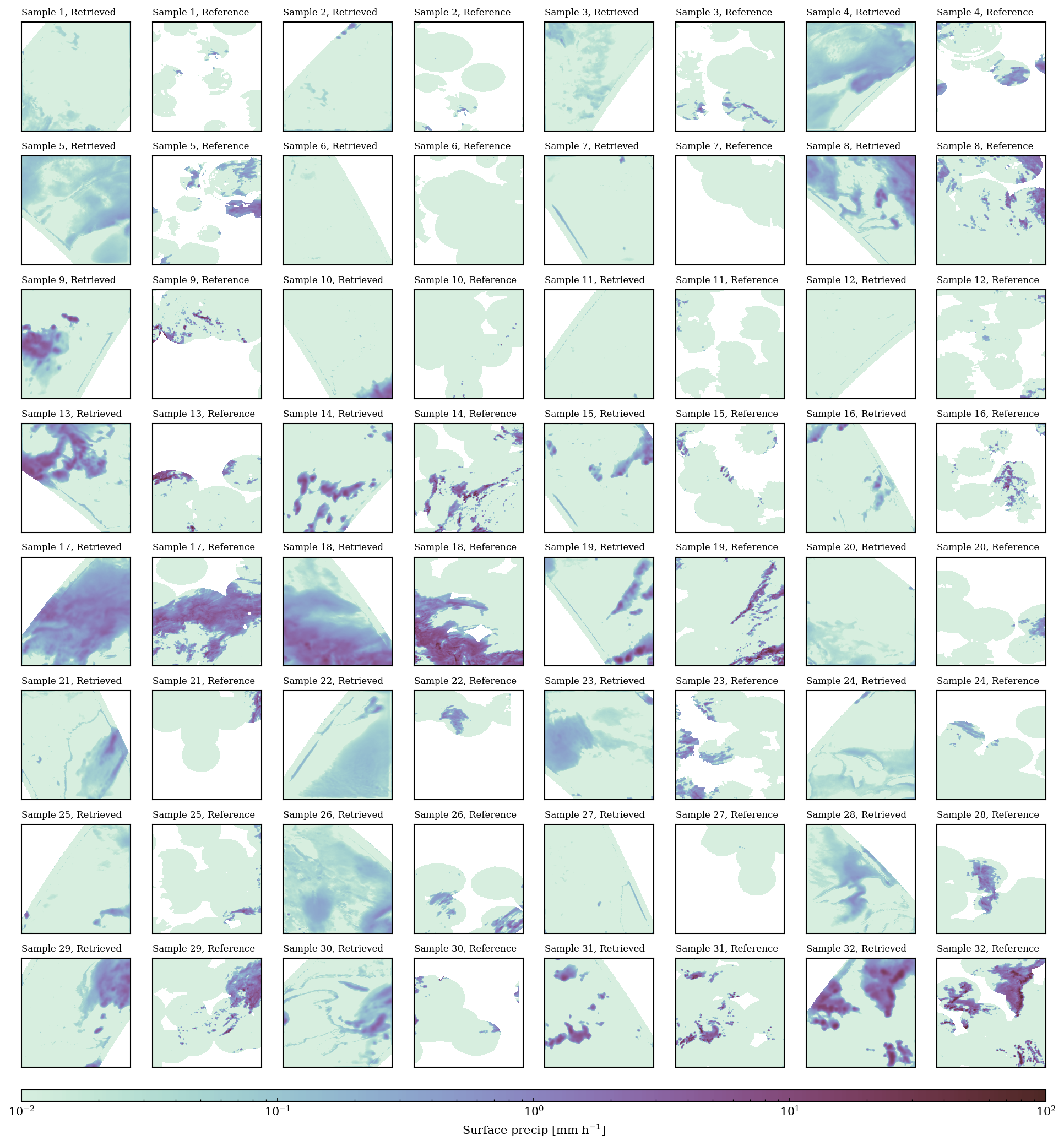
To get a first idea of how well the model works, we plot the retrieved an reference precipitation for a the first batch of samples from the validation dataset.
# Retrieve first batch from validation loader
batch = next(iter(validation_loader))
x, y = batch

x = x.to(device="cpu", dtype=torch.float32)
unet = unet.to(device="cpu", dtype=torch.float32)

# Run inference and extract surface precipitation estimates.
with torch.no_grad():
    pred = unet(x)
    surface_precip = pred["surface_precip"]
surface_precip_ref = y["surface_precip"]
from satrain.plotting import set_style, cmap_precip
import matplotlib.pyplot as plt
from matplotlib.gridspec import GridSpec
from matplotlib.colors import LogNorm
import numpy as np

set_style()
fig = plt.figure(figsize=(16, 17))
gs = GridSpec(9, 8, height_ratios = [1.0] * 8 + [0.1])

for row_ind in range(8):
    for col_ind in range(0, 8, 2):

        norm = LogNorm(1e-2, 1e2)
        sample_index = row_ind * 4 + col_ind // 2

        # Mask identifying missing values.
        mask = (x[sample_index] < -1.0).all(0)

        ax = fig.add_subplot(gs[row_ind, col_ind])
        precip = np.maximum(surface_precip[sample_index, 0].numpy().copy(), 1e-3)
        precip[mask] = np.nan
        ax.imshow(precip, norm=norm, cmap=cmap_precip)
        ax.set_xticks([])
        ax.set_yticks([])
        ax.set_title(f"Sample {sample_index + 1}, Retrieved", fontsize=8)

        ax = fig.add_subplot(gs[row_ind, col_ind + 1])
        mappable = ax.imshow(np.maximum(surface_precip_ref[sample_index], 1e-3), norm=norm, cmap=cmap_precip)
        ax.set_xticks([])
        ax.set_yticks([])
        ax.set_title(f"Sample {sample_index + 1}, Reference", fontsize=8)

cax = fig.add_subplot(gs[-1, :])
plt.colorbar(mappable, label="Surface precip [mm h$^{-1}$]", cax=cax, orientation="horizontal")
<matplotlib.colorbar.Colorbar at 0x7f9fe813f0a0>
Evaluating the retrieval#
To properly evaluate the model, we will use the test dataset. To simplify the evaluation of the UNet retrieval on the SatRain test dataset, the satrain package provides a dedicated Evaluator class that loads the input data in the format expected by the retrieval and tracks the accuracy of the retrieval results. To evaluate the retrieval using the satrain.evaluation.Evaluator class, we need to define a retrieval callback function that performes inferences on the retrieval input data provided by the evaluator. The satrain.pytorch module provides the PytorchRetrieval helper class that wraps around a trained PyTorch neural network and acts as a retrieval_fn that can be passed to the evaluator.
from satrain.pytorch import PytorchRetrieval
unet_retrieval = PytorchRetrieval(
    unet,
    retrieval_input=inputs,
    stack=True,
    device=torch.device("cpu"),
    dtype=torch.float32
)
from satrain.evaluation import Evaluator
evaluator = Evaluator(
    base_sensor="gmi",
    domain="korea",
    geometry=geometry,
    retrieval_input=inputs,
    download=True
)
Case study#
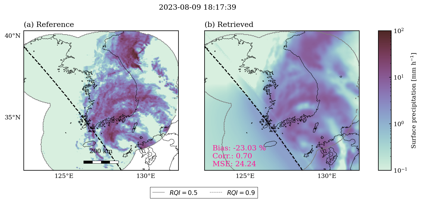
To ensure that the results returned by the UNet-based retrieval, we use the evaluator’s plot_retrieval_results function to display the results for scene 86. Passing the argument tile_size=256 ensures that the evaluator tiles the input data into tiles of size 256x256 pixels. If not explicitly specified, the overlap between neighboring tiles defaults to \(\frac{1}{4}\) of that, i.e., 64.
Since the retrieval is based on GMI observations, it will only produce reliable results where GMI observations are available. However, where this is the case the retrieval shows good agreement with the ground-based measurements.
fig = evaluator.plot_retrieval_results(
    516,
    unet_retrieval,
    input_data_format="spatial",
    tile_size=256,
    batch_size=16,
    swath_boundaries=True,
    include_metrics=True
)
Running the evaluation#
evaluator.evaluate(
    retrieval_fn=unet_retrieval,
    input_data_format="spatial",
    batch_size=32,
    n_processes=8,
    tile_size=256,
    overlap=64,
)
Results#
Precipitation estimation#
evaluator.get_precip_quantification_results(name="UNet (GMI)").T
| UNet (GMI) | ERA5 | GPROF V7 (GMI) | PERSIANN CCS | PERSIANN PDIR-Now | PU-Net | GPROF-IR | |
|---|---|---|---|---|---|---|---|
| Bias [$\%$] | -19.908477 | -12.580348 | -27.236600 | -31.790741 | -21.130333 | -6.975220 | -19.987970 |
| MAE [$mm h^{-1}$] | 0.176604 | 0.212744 | 0.338000 | 0.242497 | 0.247181 | 0.208386 | 0.172630 |
| MSE [$(mm h^{-1})^2$] | 1.914514 | 2.465700 | 5.175863 | 3.129146 | 2.917237 | 2.523134 | 1.996170 |
| SMAPE$_{0.1}$ [$\%$] | 85.906155 | 105.643559 | 83.221078 | 174.468526 | 158.385099 | 124.117068 | 87.419827 |
| Correlation coeff. [] | 0.617165 | 0.336344 | 0.650835 | 0.194232 | 0.257086 | 0.410891 | 0.566848 |
| Effective resolution [$^\circ$] | 0.569884 | inf | 0.279000 | inf | inf | inf | 1.061470 |
Precipitation detection#
evaluator.get_precip_detection_results(name="UNet (GMI)").T
| UNet (GMI) | ERA5 | GPROF V7 (GMI) | PERSIANN CCS | PERSIANN PDIR-Now | PU-Net | GPROF-IR | |
|---|---|---|---|---|---|---|---|
| POD [] | 0.535808 | NaN | 0.756630 | 0.252253 | 0.370663 | 0.634386 | 0.662734 |
| FAR [] | 0.193774 | NaN | 0.351667 | 0.607171 | 0.658323 | 0.519121 | 0.364343 |
| HSS [] | 0.795515 | NaN | 0.574699 | 0.360400 | 0.282276 | 0.423919 | 0.604062 |
Probabilistic precipitation detection#
evaluator.get_prob_precip_detection_results(name="UNet (GMI)").T
| UNet (GMI) | ERA5 | GPROF V7 (GMI) | PERSIANN CCS | PERSIANN PDIR-Now | PU-Net | GPROF-IR | |
|---|---|---|---|---|---|---|---|
| AUC [] | 0.690737 | 0.0 | 0.499888 | NaN | 0.0 | NaN | 0.613103 |
Heavy precipitation detection#
evaluator.get_heavy_precip_detection_results(name="UNet (GMI)").T
| UNet (GMI) | ERA5 | GPROF V7 (GMI) | PERSIANN CCS | PERSIANN PDIR-Now | PU-Net | GPROF-IR | |
|---|---|---|---|---|---|---|---|
| POD [] | 0.013848 | NaN | 0.756630 | 0.252253 | 0.370663 | 0.634386 | 0.662734 |
| FAR [] | 0.214869 | NaN | 0.351667 | 0.607171 | 0.658323 | 0.519121 | 0.364343 |
| HSS [] | 0.785118 | NaN | 0.574699 | 0.360400 | 0.282276 | 0.423919 | 0.604062 |
Probabilistic heavy precipitation detection#
evaluator.get_prob_heavy_precip_detection_results(name="UNet (CPCIR)").T
| UNet (CPCIR) | ERA5 | GPROF V7 (GMI) | PERSIANN CCS | PERSIANN PDIR-Now | PU-Net | GPROF-IR | |
|---|---|---|---|---|---|---|---|
| AUC [] | 0.452769 | 0.0 | 0.506518 | NaN | 0.0 | NaN | 0.292481 |